Adversarial machine learning with Flux.jl

The purpose of this tutorial is to explain how to embed a neural network model from Flux.jl into JuMP.

Required packages

This tutorial requires the following packages

using JuMP
import ExaModels
import Flux
import Ipopt
import MathOptAI
import MLDatasets
import NLPModelsIpopt
import Plots

Data

This tutorial uses images from the MNIST dataset.

We load the predefined train and test splits:

train_data = MLDatasets.MNIST(; split = :train)

dataset MNIST:
  metadata  =>    Dict{String, Any} with 3 entries
  split     =>    :train
  features  =>    28×28×60000 Array{Float32, 3}
  targets   =>    60000-element Vector{Int64}

test_data = MLDatasets.MNIST(; split = :test)

dataset MNIST:
  metadata  =>    Dict{String, Any} with 3 entries
  split     =>    :test
  features  =>    28×28×10000 Array{Float32, 3}
  targets   =>    10000-element Vector{Int64}

Since the data are images, it is helpful to plot them. (This requires a transpose and reversing the rows to get the orientation correct.)

function plot_image(x::Matrix; kwargs...)
    return Plots.heatmap(
        x'[size(x, 1):-1:1, :];
        xlims = (1, size(x, 2)),
        ylims = (1, size(x, 1)),
        aspect_ratio = true,
        legend = false,
        xaxis = false,
        yaxis = false,
        kwargs...,
    )
end

function plot_image(instance::NamedTuple)
    return plot_image(instance.features; title = "Label = $(instance.targets)")
end

Plots.plot([plot_image(train_data[i]) for i in 1:6]...; layout = (2, 3))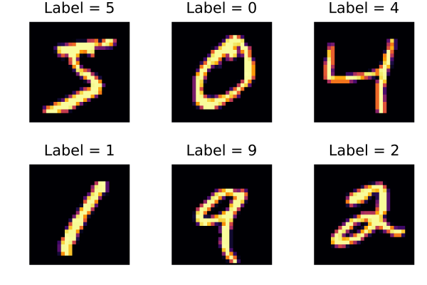

Training

We use a simple neural network with one hidden layer and a sigmoid activation function. (There are better performing networks; try experimenting.)

predictor = Flux.Chain(
    Flux.Dense(28^2 => 32, Flux.sigmoid),
    Flux.Dense(32 => 10),
    Flux.softmax,
)

Chain(
  Dense(784 => 32, σ),                  # 25_120 parameters
  Dense(32 => 10),                      # 330 parameters
  NNlib.softmax,
)                   # Total: 4 arrays, 25_450 parameters, 99.617 KiB.

Here is a function to load our data into the format that predictor expects:

function data_loader(data; batchsize, shuffle = false)
    x = reshape(data.features, 28^2, :)
    y = Flux.onehotbatch(data.targets, 0:9)
    return Flux.DataLoader((x, y); batchsize, shuffle)
end

data_loader (generic function with 1 method)

and here is a function to score the percentage of correct labels, where we assign a label by choosing the label of the highest softmax in the final layer.

function score_model(predictor, data)
    x, y = only(data_loader(data; batchsize = length(data)))
    y_hat = predictor(x)
    is_correct = Flux.onecold(y) .== Flux.onecold(y_hat)
    p = round(100 * sum(is_correct) / length(is_correct); digits = 2)
    println("Accuracy = $p %")
    return
end

score_model (generic function with 1 method)

The accuracy of our model is only around 10% before training:

score_model(predictor, train_data)
score_model(predictor, test_data)

Accuracy = 9.96 %
Accuracy = 9.88 %

Let's improve that by training our model.

begin
    train_loader = data_loader(train_data; batchsize = 256, shuffle = true)
    optimizer_state = Flux.setup(Flux.Adam(3e-4), predictor)
    for epoch in 1:30
        loss = 0.0
        for (x, y) in train_loader
            loss_batch, gradient = Flux.withgradient(predictor) do model
                return Flux.crossentropy(model(x), y)
            end
            Flux.update!(optimizer_state, predictor, only(gradient))
            loss += loss_batch
        end
        loss = round(loss / length(train_loader); digits = 4)
        print("Epoch $epoch: loss = $loss\t")
        score_model(predictor, test_data)
    end
end

Epoch 1: loss = 1.7815	Accuracy = 75.37 %
Epoch 2: loss = 1.1542	Accuracy = 83.29 %
Epoch 3: loss = 0.8572	Accuracy = 86.9 %
Epoch 4: loss = 0.6812	Accuracy = 88.41 %
Epoch 5: loss = 0.5686	Accuracy = 89.51 %
Epoch 6: loss = 0.4931	Accuracy = 90.12 %
Epoch 7: loss = 0.4402	Accuracy = 90.54 %
Epoch 8: loss = 0.4014	Accuracy = 90.93 %
Epoch 9: loss = 0.3715	Accuracy = 91.26 %
Epoch 10: loss = 0.3472	Accuracy = 91.68 %
Epoch 11: loss = 0.3277	Accuracy = 91.93 %
Epoch 12: loss = 0.3118	Accuracy = 92.07 %
Epoch 13: loss = 0.298	Accuracy = 92.35 %
Epoch 14: loss = 0.2861	Accuracy = 92.47 %
Epoch 15: loss = 0.2754	Accuracy = 92.67 %
Epoch 16: loss = 0.2663	Accuracy = 92.85 %
Epoch 17: loss = 0.2575	Accuracy = 92.93 %
Epoch 18: loss = 0.2496	Accuracy = 93.16 %
Epoch 19: loss = 0.2426	Accuracy = 93.33 %
Epoch 20: loss = 0.2358	Accuracy = 93.46 %
Epoch 21: loss = 0.2297	Accuracy = 93.67 %
Epoch 22: loss = 0.2238	Accuracy = 93.65 %
Epoch 23: loss = 0.2183	Accuracy = 93.75 %
Epoch 24: loss = 0.2134	Accuracy = 93.81 %
Epoch 25: loss = 0.2087	Accuracy = 93.95 %
Epoch 26: loss = 0.2045	Accuracy = 94.12 %
Epoch 27: loss = 0.1998	Accuracy = 94.17 %
Epoch 28: loss = 0.1959	Accuracy = 94.24 %
Epoch 29: loss = 0.1924	Accuracy = 94.3 %
Epoch 30: loss = 0.1889	Accuracy = 94.45 %

Here are the first eight predictions of the test data:

function plot_image(predictor, x::Matrix)
    score, index = findmax(predictor(vec(x)))
    title = "Predicted: $(index - 1) ($(round(Int, 100 * score))%)"
    return plot_image(x; title)
end

plots = [plot_image(predictor, test_data[i].features) for i in 1:8]
Plots.plot(plots...; size = (1200, 600), layout = (2, 4))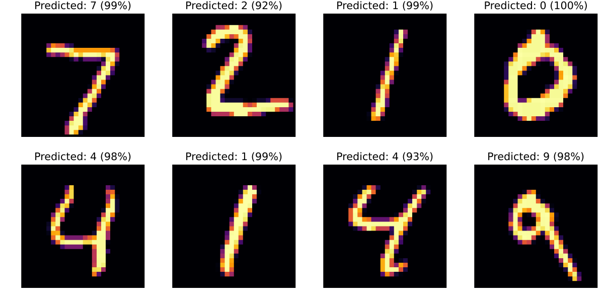

We can also look at the best and worst four predictions:

x, y = only(data_loader(test_data; batchsize = length(test_data)))
losses = Flux.crossentropy(predictor(x), y; agg = identity)
indices = sortperm(losses; dims = 2)[[1:4; (end-3):end]]
plots = [plot_image(predictor, test_data[i].features) for i in indices]
Plots.plot(plots...; size = (1200, 600), layout = (2, 4))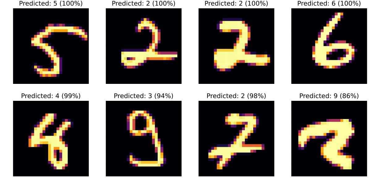

There are still some fairly bad mistakes. Can you change the model or training parameters improve to improve things?

JuMP

Now that we have a trained machine learning model, we can embed it in a JuMP model.

Here's a function which takes a test case and returns an example that maximizes the probability of the adversarial example.

function find_adversarial_image(test_case; adversary_label, δ = 0.05)
    model = Model(Ipopt.Optimizer)
    set_silent(model)
    @variable(model, 0 <= x[1:28, 1:28] <= 1)
    @constraint(model, -δ .<= x .- test_case.features .<= δ)
    # Note: we need to use `vec` here because `x` is a 28-by-28 Matrix, but our
    # neural network expects a 28^2 length vector.
    y, _ = MathOptAI.add_predictor(model, predictor, vec(x))
    @objective(model, Max, y[adversary_label+1] - y[test_case.targets+1])
    optimize!(model)
    @assert is_solved_and_feasible(model)
    return value.(x)
end

find_adversarial_image (generic function with 1 method)

Let's try finding an adversarial example to the third test image. The image on the left is our input image. The network thinks this is a 1 with probability 99%. The image on the right is the adversarial image. The network thinks this is a 7, although it is less confident.

x_adversary = find_adversarial_image(test_data[3]; adversary_label = 7);
Plots.plot(
    plot_image(predictor, test_data[3].features),
    plot_image(predictor, Float32.(x_adversary)),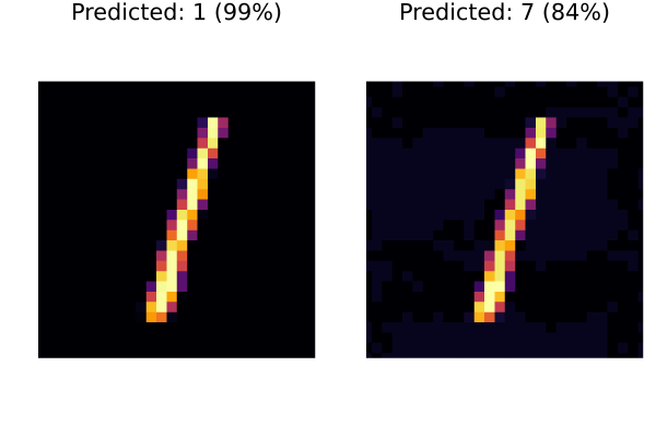
)

ExaModels

We can do a similar thing with ExaModels:

function find_adversarial_image_exa(test_case; adversary_label, δ = 0.05)
    core = ExaModels.ExaCore(; concrete = Val(true))
    core, x = ExaModels.add_var(core, 28^2; lvar = 0, uvar = 1)
    core, _ = ExaModels.add_con(
        core,
        x[i] - f for (i, f) in enumerate(test_case.features);
        lcon = -δ,
        ucon = δ,
    )
    (core, y), _ = MathOptAI.add_predictor(core, predictor, x)
    core, _ =
        ExaModels.add_obj(core, y[test_case.targets+1] - y[adversary_label+1])
    model = ExaModels.ExaModel(core)
    result = NLPModelsIpopt.ipopt(model; print_level = 0)
    @assert result.status ∈ (:first_order, :acceptable)
    x = ExaModels.solution(result, x)
    return reshape(x, 28, 28)
end

x_adversary = find_adversarial_image_exa(test_data[3]; adversary_label = 7)
Plots.plot(
    plot_image(predictor, test_data[3].features),
    plot_image(predictor, Float32.(x_adversary)),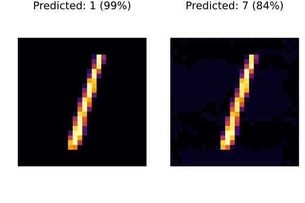
)

This page was generated using Literate.jl.