Adversarial machine learning with Lux.jl

The purpose of this tutorial is to explain how to embed a neural network model from Lux.jl into JuMP.

Required packages

This tutorial requires the following packages

using JuMP
import Lux
import Ipopt
import MathOptAI
import MLDatasets
import MLUtils
import OneHotArrays
import Optimisers
import Plots
import Random
import Zygote

Data

This tutorial uses images from the MNIST dataset.

We load the predefined train and test splits:

train_data = MLDatasets.MNIST(; split = :train)

dataset MNIST:
  metadata  =>    Dict{String, Any} with 3 entries
  split     =>    :train
  features  =>    28×28×60000 Array{Float32, 3}
  targets   =>    60000-element Vector{Int64}

test_data = MLDatasets.MNIST(; split = :test)

dataset MNIST:
  metadata  =>    Dict{String, Any} with 3 entries
  split     =>    :test
  features  =>    28×28×10000 Array{Float32, 3}
  targets   =>    10000-element Vector{Int64}

Since the data are images, it is helpful to plot them. (This requires a transpose and reversing the rows to get the orientation correct.)

function plot_image(x::Matrix; kwargs...)
    return Plots.heatmap(
        x'[size(x, 1):-1:1, :];
        xlims = (1, size(x, 2)),
        ylims = (1, size(x, 1)),
        aspect_ratio = true,
        legend = false,
        xaxis = false,
        yaxis = false,
        kwargs...,
    )
end

function plot_image(instance::NamedTuple)
    return plot_image(instance.features; title = "Label = $(instance.targets)")
end

Plots.plot([plot_image(train_data[i]) for i in 1:6]...; layout = (2, 3))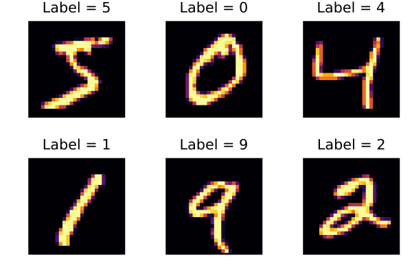

Training

We use a simple neural network with one hidden layer and a sigmoid activation function. (There are better performing networks; try experimenting.)

chain = Lux.Chain(
    Lux.Dense(28^2 => 32, Lux.sigmoid),
    Lux.Dense(32 => 10),
    Lux.softmax,
)
rng = Random.MersenneTwister();
parameters, state = Lux.setup(rng, chain)
predictor = (chain, parameters, state);

Here is a function to load our data into the format that predictor expects:

function data_loader(data; batchsize, shuffle = false)
    x = reshape(data.features, 28^2, :)
    y = OneHotArrays.onehotbatch(data.targets, 0:9)
    return MLUtils.DataLoader((x, y); batchsize, shuffle)
end

data_loader (generic function with 1 method)

and here is a function to score the percentage of correct labels, where we assign a label by choosing the label of the highest softmax in the final layer.

function score_model(predictor, data)
    chain, parameters, state = predictor
    x, y = only(data_loader(data; batchsize = length(data)))
    y_hat, _ = chain(x, parameters, state)
    is_correct = OneHotArrays.onecold(y) .== OneHotArrays.onecold(y_hat)
    p = round(100 * sum(is_correct) / length(is_correct); digits = 2)
    println("Accuracy = $p %")
    return
end

score_model (generic function with 1 method)

The accuracy of our model is only around 10% before training:

score_model(predictor, train_data)
score_model(predictor, test_data)

Accuracy = 7.02 %
Accuracy = 7.3 %

Let's improve that by training our model.

begin
    train_loader = data_loader(train_data; batchsize = 256, shuffle = true)
    optimizer_state = Optimisers.setup(Optimisers.Adam(0.0003f0), parameters)
    for epoch in 1:30
        loss = 0.0
        for (x, y) in train_loader
            global state
            (loss_batch, state), pullback = Zygote.pullback(parameters) do p
                y_model, new_state = chain(x, p, state)
                return Lux.CrossEntropyLoss()(y_model, y), new_state
            end
            gradients = only(pullback((one(loss), nothing)))
            Optimisers.update!(optimizer_state, parameters, gradients)
            loss += loss_batch
        end
        loss = round(loss / length(train_loader); digits = 4)
        print("Epoch $epoch: loss = $loss\t")
        score_model(predictor, test_data)
    end
end

Epoch 1: loss = 1.8588	Accuracy = 80.36 %
Epoch 2: loss = 1.2434	Accuracy = 84.91 %
Epoch 3: loss = 0.914	Accuracy = 86.95 %
Epoch 4: loss = 0.719	Accuracy = 88.13 %
Epoch 5: loss = 0.5964	Accuracy = 89.19 %
Epoch 6: loss = 0.5144	Accuracy = 89.83 %
Epoch 7: loss = 0.4571	Accuracy = 90.33 %
Epoch 8: loss = 0.4147	Accuracy = 90.84 %
Epoch 9: loss = 0.3825	Accuracy = 91.21 %
Epoch 10: loss = 0.3571	Accuracy = 91.43 %
Epoch 11: loss = 0.3364	Accuracy = 91.7 %
Epoch 12: loss = 0.3195	Accuracy = 91.85 %
Epoch 13: loss = 0.3049	Accuracy = 92.05 %
Epoch 14: loss = 0.2923	Accuracy = 92.39 %
Epoch 15: loss = 0.2817	Accuracy = 92.45 %
Epoch 16: loss = 0.2718	Accuracy = 92.7 %
Epoch 17: loss = 0.2635	Accuracy = 92.9 %
Epoch 18: loss = 0.2557	Accuracy = 92.96 %
Epoch 19: loss = 0.2486	Accuracy = 93.15 %
Epoch 20: loss = 0.2422	Accuracy = 93.16 %
Epoch 21: loss = 0.2362	Accuracy = 93.28 %
Epoch 22: loss = 0.2305	Accuracy = 93.47 %
Epoch 23: loss = 0.2254	Accuracy = 93.58 %
Epoch 24: loss = 0.2207	Accuracy = 93.65 %
Epoch 25: loss = 0.2157	Accuracy = 93.78 %
Epoch 26: loss = 0.2116	Accuracy = 93.85 %
Epoch 27: loss = 0.2075	Accuracy = 93.91 %
Epoch 28: loss = 0.2032	Accuracy = 93.99 %
Epoch 29: loss = 0.1996	Accuracy = 94.08 %
Epoch 30: loss = 0.1961	Accuracy = 94.11 %

Here are the first eight predictions of the test data:

function plot_image(predictor, x::Matrix)
    y, _ = chain(vec(x), parameters, state)
    score, index = findmax(y)
    title = "Predicted: $(index - 1) ($(round(Int, 100 * score))%)"
    return plot_image(x; title)
end

plots = [plot_image(predictor, test_data[i].features) for i in 1:8]
Plots.plot(plots...; size = (1200, 600), layout = (2, 4))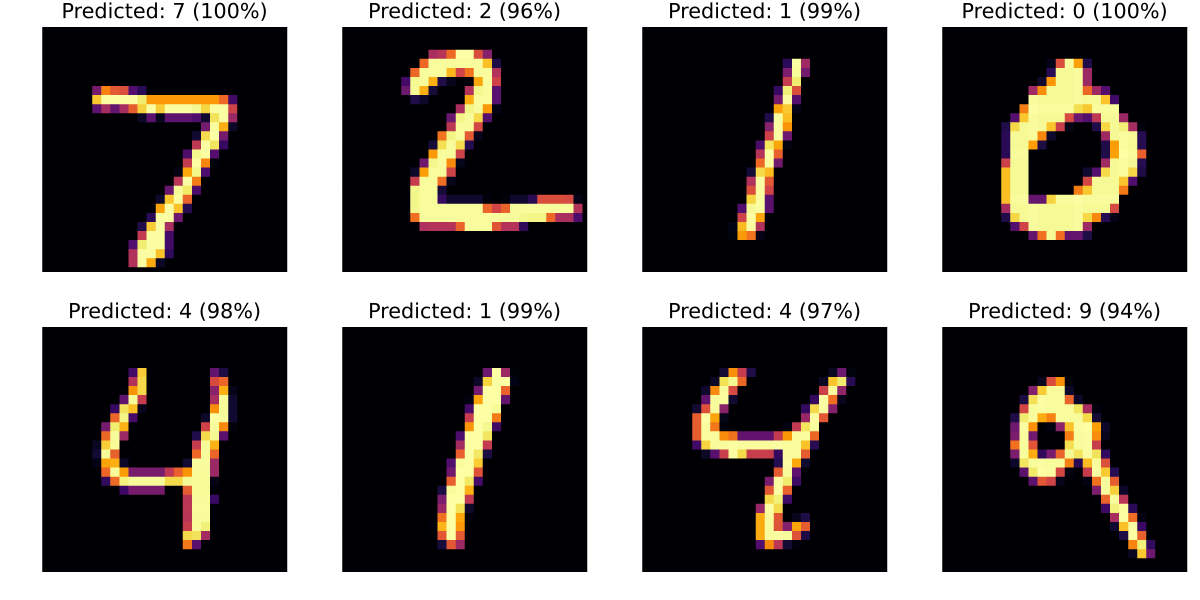

We can also look at the best and worst four predictions:

x, y = only(data_loader(test_data; batchsize = length(test_data)))
y_model, _ = chain(x, parameters, state)
losses = Lux.CrossEntropyLoss(; agg = identity)(y_model, y)
indices = sortperm(losses; dims = 2)[[1:4; (end-3):end]]
plots = [plot_image(predictor, test_data[i].features) for i in indices]
Plots.plot(plots...; size = (1200, 600), layout = (2, 4))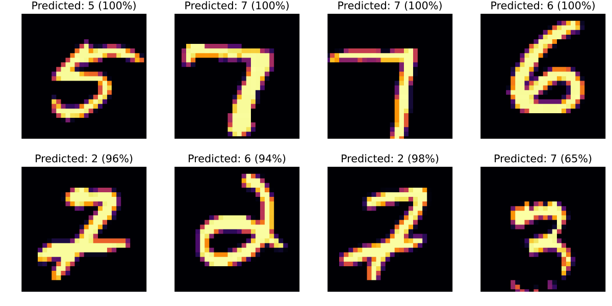

There are still some fairly bad mistakes. Can you change the model or training parameters improve to improve things?

JuMP

Now that we have a trained machine learning model, we can embed it in a JuMP model.

Here's a function which takes a test case and returns an example that maximizes the probability of the adversarial example.

function find_adversarial_image(test_case; adversary_label, δ = 0.05)
    model = Model(Ipopt.Optimizer)
    set_silent(model)
    @variable(model, 0 <= x[1:28, 1:28] <= 1)
    @constraint(model, -δ .<= x .- test_case.features .<= δ)
    # Note: we need to use `vec` here because `x` is a 28-by-28 Matrix, but our
    # neural network expects a 28^2 length vector.
    y, _ = MathOptAI.add_predictor(model, predictor, vec(x))
    @objective(model, Max, y[adversary_label+1] - y[test_case.targets+1])
    optimize!(model)
    @assert is_solved_and_feasible(model)
    return value.(x)
end

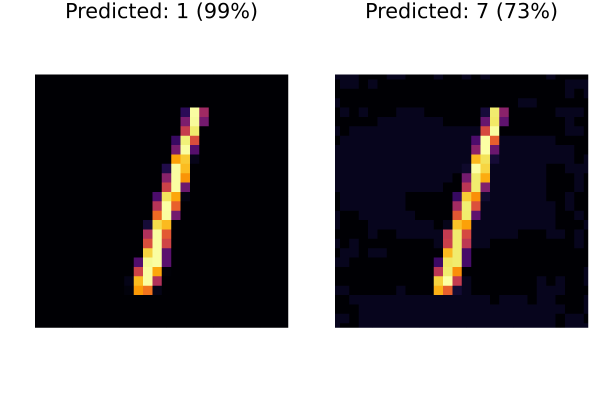
find_adversarial_image (generic function with 1 method)

Let's try finding an adversarial example to the third test image. The image on the left is our input image. The network thinks this is a 1 with probability 99%. The image on the right is the adversarial image. The network thinks this is a 7, although it is less confident.

x_adversary = find_adversarial_image(test_data[3]; adversary_label = 7);
Plots.plot(
    plot_image(predictor, test_data[3].features),
    plot_image(predictor, Float32.(x_adversary)),
)

This page was generated using Literate.jl.